 Rohit Gupta
Integrating single-cell RNA-seq with scVI
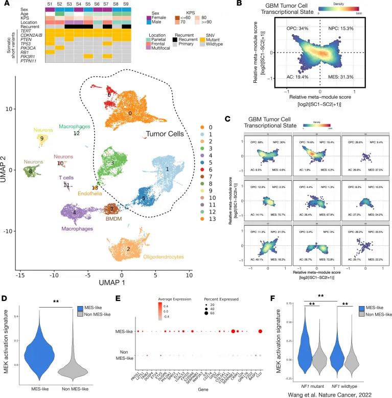
Single-cell studies of brain tumors often sample the same disease more than once: a primary tumor and its recurrence, from several patients, sometimes processed months or years apart with different chemistry versions. Put all of that into one AnnData, run PCA and UMAP, and you mostly get a map of who was sequenced when. Cells cluster by sample before they cluster by cell type.
Integration is the step that tries to fix that: put cells from different batches into a shared space where the same cell type lands in the same place, without erasing real differences. My default tool for it is scVI from scvi-tools. This post walks through a full workflow on a public dataset that ships with scvi-tools, so every block runs as written.
Why integration is needed
Technical and biological nuisance factors stack up quickly in single-cell data:
- Batch: library preparation day, sequencing run, operator.
- Chemistry and protocol: 10x 3’ v2 vs v3, single cells vs single nuclei, enrichment protocols.
- Donor or patient: genetics, age, sex, treatment history.
These effects are not small corrections. They change which genes are detected and at what level, often more than the difference between closely related cell states. Without integration you either analyze each sample separately or accept clusters that partly reflect processing.
The flip side is that some of these factors are also biology. Patient-to-patient differences in tumor cells are real, and they are often the point of the study. Integration is always a decision about what you are willing to remove, and I come back to that at the end.
What scVI does
scVI (Lopez et al., 2018) is a variational autoencoder for count data. The parts that matter in practice:
- It models raw counts directly with a negative binomial (or zero-inflated negative binomial) likelihood, and it accounts for library size, so you do not feed it log-normalized data.
- An encoder network maps each cell’s expression to a low-dimensional latent vector, typically 10 to 30 dimensions.
- A decoder network maps the latent vector, together with the cell’s batch, back to parameters of the count distribution. Because the decoder is told the batch, the latent space does not need to encode it, and batch variation is pushed out of the latent representation. (The encoder can optionally see batch too.)
- Because it is a generative model, the same fitted model gives you an integrated embedding, batch-corrected and denoised expression values, and a framework for differential expression.
scvi-tools (Gayoso et al., 2022) is the library that packages scVI along with related models such as scANVI, which I use below for label transfer.
Setup
pip install scvi-tools "scanpy[leiden]" scikit-misc scib-metrics
scikit-misc is needed for flavor="seurat_v3" highly variable gene selection, and the leiden extra pulls in igraph and leidenalg. If you have an NVIDIA GPU, install a CUDA build of PyTorch first by following the PyTorch instructions; scvi-tools picks it up automatically.
The example data
scvi.data.heart_cell_atlas_subsampled() downloads a subsample of the adult human heart cell atlas: a little under 20,000 cells from multiple donors, profiled with four different protocols (single nuclei from two sites, single cells, and CD45-enriched cells). It has the same structure as my tumor problem: several donors, more than one protocol, and cell type labels you can use to check whether integration preserved biology.
import numpy as np
import pandas as pd
import scanpy as sc
import scvi
import torch

scvi.settings.seed = 0
torch.set_float32_matmul_precision("high")

adata = scvi.data.heart_cell_atlas_subsampled(save_path="data/")
adata
The columns I use are cell_source (the protocol), donor and cell_type.
adata.obs["cell_source"].value_counts()
pd.crosstab(adata.obs["donor"], adata.obs["cell_source"])
The crosstab is worth looking at for any dataset. If a batch contains only one donor, or one cell type exists only in one batch, the model cannot separate those factors, and you should know that before you trust the result.
Quality control
adata.X in this dataset holds raw counts, which is what scVI needs. The dataset was already filtered by its authors, and by default the loader also removes clusters annotated as doublets or unassigned cells. On your own data you would do the usual QC first:
adata.var["mt"] = adata.var_names.str.startswith("MT-")
sc.pp.calculate_qc_metrics(
    adata, qc_vars=["mt"], percent_top=None, log1p=False, inplace=True
)
sc.pl.violin(
    adata,
    ["n_genes_by_counts", "total_counts", "pct_counts_mt"],
    groupby="cell_source",
    rotation=45,
)
Look at these distributions per batch before choosing cutoffs. Single-nucleus data has very little mitochondrial RNA by construction, while some intact cell types (cardiomyocytes are an extreme example) are naturally mitochondria-rich. One global mitochondrial threshold across protocols will remove the wrong cells.
For your own data, the filtering step looks like this. The thresholds are placeholders to be set from your own plots:
# On your own data (placeholder thresholds):
# sc.pp.filter_cells(adata, min_genes=200)
# adata = adata[adata.obs["pct_counts_mt"] < 10].copy()
Doublets. Run doublet detection per sample on raw counts before integration. sc.pp.scrublet(adata, batch_key="sample") runs Scrublet within each sample, and scvi-tools has its own doublet model, SOLO (scvi.external.SOLO), that is trained on top of an scVI model. Doublets that survive tend to form small “bridge” clusters between cell types after integration.
Then remove genes that are almost never detected and keep a copy of the counts:
sc.pp.filter_genes(adata, min_counts=3)

adata.layers["counts"] = adata.X.copy()   # scVI will read from here
sc.pp.normalize_total(adata, target_sum=1e4)
sc.pp.log1p(adata)
adata.raw = adata                         # full log-normalized matrix for plotting
From here, adata.X is log-normalized (for PCA and plotting) and adata.layers["counts"] holds the raw counts for scVI. Keeping these straight prevents the most common scVI mistake, which is training on normalized data.
Highly variable genes
sc.pp.highly_variable_genes(
    adata,
    n_top_genes=2000,
    flavor="seurat_v3",
    layer="counts",
    batch_key="cell_source",
    subset=True,
)
Two details matter here. flavor="seurat_v3" expects raw counts, hence layer="counts". And batch_key selects genes that are variable within batches rather than genes that differ between batches, so you do not select the batch effect itself as your feature set. Somewhere between 2,000 and 4,000 genes is typical; more genes mean slower training and rarely much better integration.
subset=True keeps only those genes in adata. The full gene set is still in adata.raw for plotting.
Setting up and training the model
setup_anndata registers which data the model uses:
scvi.model.SCVI.setup_anndata(
    adata,
    layer="counts",
    batch_key="cell_source",
    categorical_covariate_keys=["donor"],
)
batch_key is the main factor to integrate over. categorical_covariate_keys adds further discrete nuisance factors (here donor), and continuous_covariate_keys exists for things like mitochondrial fraction. A common alternative is to build a single combined key, for example protocol and donor pasted together, and pass that as batch_key. Either way, only include factors you actually want removed from the latent space.
model = scvi.model.SCVI(
    adata,
    n_latent=30,
    n_layers=2,
    gene_likelihood="nb",
)
model
The defaults are n_latent=10, n_layers=1 and gene_likelihood="zinb". For integration across several batches I usually go with a slightly larger model: 2 layers and 30 latent dimensions. The negative binomial likelihood is usually sufficient for UMI data. These are reasonable starting points, not tuned values.
model.train(
    max_epochs=400,
    early_stopping=True,
    early_stopping_patience=20,
    check_val_every_n_epoch=1,
    accelerator="auto",
)
If you leave out max_epochs, scvi-tools picks a number based on dataset size (fewer epochs for larger datasets, capped at 400). By default 10% of cells are held out for validation, and early_stopping=True stops training when the validation ELBO stops improving. Check the training curves:
import matplotlib.pyplot as plt

hist = model.history
fig, ax = plt.subplots(figsize=(6, 4))
ax.plot(hist["elbo_train"], label="train")
ax.plot(hist["elbo_validation"], label="validation")
ax.set_xlabel("epoch")
ax.set_ylabel("ELBO")
ax.legend()
plt.show()
You want both curves flattening out together. A validation curve that rises while training keeps falling means overfitting; a curve still dropping steeply at the end means training stopped too early.
Latent space, neighbors, UMAP and clusters
To see what integration bought you, first make an uncorrected baseline from PCA on the log-normalized data:
sc.tl.pca(adata)
sc.pp.neighbors(adata, use_rep="X_pca")
sc.tl.umap(adata)
adata.obsm["X_umap_pca"] = adata.obsm["X_umap"].copy()
Then compute the same graph on the scVI latent space:
adata.obsm["X_scVI"] = model.get_latent_representation()

sc.pp.neighbors(adata, use_rep="X_scVI")
sc.tl.umap(adata, min_dist=0.3)
sc.tl.leiden(
    adata,
    key_added="leiden_scVI",
    resolution=0.5,
    flavor="igraph",
    n_iterations=2,
    directed=False,
)
sc.pl.embedding(adata, basis="X_umap_pca", color=["cell_source", "cell_type"], ncols=2)
sc.pl.umap(adata, color=["cell_source", "donor", "cell_type", "leiden_scVI"], ncols=2)
The neighbor graph, UMAP and Leiden clusters now all come from the scVI embedding. Everything downstream that depends on the graph (clustering, trajectory methods, label propagation) should use X_scVI, not PCA.
Batch-corrected expression
The latent space is for structure. For gene-level questions, the model can also produce normalized expression values:
adata.layers["scvi_normalized"] = model.get_normalized_expression(
    library_size=1e4, return_numpy=True
)
These are the model’s estimated expression frequencies for each cell, scaled to 10,000 counts. They are smoothed, which makes marker plots and heatmaps much cleaner. You can also ask for expression as if every cell had come from one batch, with transform_batch="Sanger-Cells", for example.
Two cautions. These values are model outputs, not measurements, so do not feed them into a standard statistical test as if each cell were an independent observation. And smoothing can make a gene look expressed in a population where it is barely detected; check the raw detection rate when it matters.
Differential expression
scVI has its own Bayesian differential expression built on the generative model:
de = model.differential_expression(
    groupby="cell_type",
    group1="Endothelial",
    group2="Fibroblast",
    mode="change",       # test for a change bigger than delta, not just any change
    delta=0.25,          # minimum effect size on the log fold change scale
    fdr_target=0.05,     # adds the is_de_fdr_0.05 column used below
)

top = de[de["is_de_fdr_0.05"]].sort_values("lfc_mean", ascending=False)
top[["lfc_mean", "bayes_factor", "proba_de",
     "non_zeros_proportion1", "non_zeros_proportion2"]].head(10)
The result is a data frame indexed by gene. lfc_mean is the estimated log fold change, proba_de is the posterior probability that the change exceeds a minimum effect size, is_de_fdr_0.05 flags genes passing a posterior-based FDR control at 5%, and non_zeros_proportion1 and non_zeros_proportion2 give raw detection rates in each group. Leaving out group1 and group2 gives one-vs-rest comparisons for every category, which is a quick way to get marker candidates. batch_correction=True averages over batches when computing expression, which helps when your groups are unevenly distributed across batches.
For comparisons between conditions, such as primary vs recurrent tumors, keep in mind that the replicate is the patient, not the cell. Model-based DE on thousands of cells from a few patients will happily report tiny p-values for differences driven by one patient. For condition-level claims I use the scVI embedding to define cell populations and then test with pseudobulk counts per patient.
Label transfer with scANVI
Often you have labels for part of the data: a reference you annotated carefully, or published annotations for some samples, plus new samples without labels. scANVI (Xu et al., 2021) extends scVI with a cell type label that can be missing for some cells. It uses the labeled cells to shape the latent space and predicts labels for the rest.
To simulate this, hide the labels of a few donors:
held_out = adata.obs["donor"].unique()[:3]
mask = adata.obs["donor"].isin(held_out)

adata.obs["cell_type_partial"] = adata.obs["cell_type"].astype(str)
adata.obs.loc[mask, "cell_type_partial"] = "Unknown"
The recommended way to train scANVI is to start from a trained scVI model:
scanvi_model = scvi.model.SCANVI.from_scvi_model(
    model,
    unlabeled_category="Unknown",
    labels_key="cell_type_partial",
    adata=adata,
)
scanvi_model.train(max_epochs=20, n_samples_per_label=100)

adata.obsm["X_scANVI"] = scanvi_model.get_latent_representation()
adata.obs["scanvi_pred"] = scanvi_model.predict()

probs = scanvi_model.predict(soft=True)          # data frame, one column per label
adata.obs["scanvi_max_prob"] = probs.max(axis=1).values
Because we hid labels we actually have, we can check the predictions on the held-out donors:
pd.crosstab(
    adata.obs.loc[mask, "cell_type"],
    adata.obs.loc[mask, "scanvi_pred"],
)
On real data, look at scanvi_max_prob: low-confidence cells are often doublets, transitional states or cell types absent from the labeled set. scANVI can only assign labels it has seen, so a new tumor-specific population will be forced into the closest known label. Treat predictions as a starting annotation that you confirm with markers.
The same machinery supports reference mapping: you train on a reference, then add new query data to the trained model without retraining from scratch (prepare_query_anndata and load_query_data on the model class). That is the scArches approach, and it is handy when new samples keep arriving.
Saving and loading models
model.save("models/heart_scvi", overwrite=True)
scanvi_model.save("models/heart_scanvi", overwrite=True)
adata.write_h5ad("heart_integrated.h5ad")

# Later
adata = sc.read_h5ad("heart_integrated.h5ad")
model = scvi.model.SCVI.load("models/heart_scvi", adata=adata)
load checks that the AnnData has the same genes and the setup fields the model was trained with. Save the model and the AnnData together, and record the package versions: a small text file with scvi.__version__ and the setup arguments next to each model directory is enough.
GPU vs CPU
scVI trains on CPU, but slowly. On a dataset like this one a CPU is workable; for anything in the hundreds of thousands of cells, use a GPU.
torch.cuda.is_available() # True if PyTorch can see an NVIDIA GPU
accelerator="auto" uses a GPU when one is available. You can force a choice with accelerator="gpu", devices=1 or accelerator="cpu". On recent Macs, accelerator="mps" may work, but support depends on your PyTorch version, so I check for warnings when using it. Increasing batch_size in train() (the default is 128) speeds up GPU training on large datasets, at the cost of fewer optimization steps per epoch.
Judging integration
There are two ways to fail. Under-correction: cells still separate by batch within a cell type. Over-correction: cells that are biologically different get merged because the model treated the difference as batch. The second is harder to spot because the UMAP looks nice.
What I check:
- Color the UMAP by batch and by cell type. Within a cell type, batches should intermix. Across cell types, separation should remain.
-
Look at batch composition per cluster, not just the picture:
 pd.crosstab(
     adata.obs["leiden_scVI"],
     adata.obs["cell_source"],
     normalize="index",
 ).round(2)
Perfect mixing everywhere is not the goal. In this dataset the CD45-enriched protocol should be over-represented in immune clusters, because that is what the enrichment does. If immune cells from that protocol were spread evenly across all clusters, that would be over-correction.
- Check markers per cluster. Clusters should still have coherent marker genes. Clusters defined only by batch-specific genes, or with mixed markers from two lineages, are warning signs.
- Compare against the uncorrected baseline. If a cell type is distinct in the PCA embedding within each batch and merges with another after integration, find out why.
-
Quantify. scib-metrics (based on the benchmarking framework in Luecken et al., 2022) computes batch-mixing and biology-conservation metrics for several embeddings at once:
 from scib_metrics.benchmark import Benchmarker

 bm = Benchmarker(
     adata,
     batch_key="cell_source",
     label_key="cell_type",
     embedding_obsm_keys=["X_pca", "X_scVI", "X_scANVI"],
     n_jobs=4,
 )
 bm.benchmark()
 bm.plot_results_table(min_max_scale=False)
One caveat: scANVI was trained using most of these same labels, so its biology-conservation scores are optimistic here. Metrics need labels you trust, and the metric suite rewards mixing that may not be appropriate for your design.
For tumor data specifically, the batch definition is the main decision. Malignant cells from different patients differ for real reasons (different copy number changes, different driver mutations), and integrating on patient can blend distinct malignant programs into shared clusters. A reasonable pattern is to integrate on technical factors (protocol, chemistry, run) and look at malignant cells both with and without patient as a covariate, and to annotate non-malignant cells, where cross-patient mixing is expected, on the fully integrated embedding.
Checklist
- Keep raw counts in
adata.layers["counts"]and confirm they are integers before training. - QC per batch, remove doublets per sample, and look at the batch by donor by cell type crosstab.
- Select 2,000 to 4,000 HVGs with
flavor="seurat_v3",layer="counts"andbatch_key. setup_anndatawith only the factors you want removed; start withn_latent=30,n_layers=2,gene_likelihood="nb".- Train with early stopping and check the training curves.
- Build neighbors, UMAP and clusters on
X_scVI. - Judge integration with batch composition, markers, a PCA baseline and, if you have trusted labels, scib-metrics.
- Use scANVI when you have partial labels; review low-confidence predictions.
- Use pseudobulk per patient for condition-level differential expression.
- Save the model, the AnnData and the package versions together.
The scvi-tools documentation has tutorials for most of the models mentioned here, including reference mapping and multimodal models such as totalVI for CITE-seq.
References
- Gayoso A, et al. A Python library for probabilistic analysis of single-cell omics data. Nature Biotechnology 40, 163-166 (2022).
- Lopez R, et al. Deep generative modeling for single-cell transcriptomics. Nature Methods 15, 1053-1058 (2018).
- Luecken MD, et al. Benchmarking atlas-level data integration in single-cell genomics. Nature Methods 19, 41-50 (2022).
- Wolf FA, et al. SCANPY: large-scale single-cell gene expression data analysis. Genome Biology 19, 15 (2018).
- Xu C, et al. Probabilistic harmonization and annotation of single-cell transcriptomics data with deep generative models. Molecular Systems Biology 17, e9620 (2021).